
Back to the Register: Distilling the Federal Register for All
Published on:Table of Contents
Introduction
A year and a half ago, I wrote Federal Register Data Exploration with R, and I had written it mainly for myself, as a way of exhibiting a technique I called “flexml” (a portmanteau of flexible and xml). The post is light on details about how to transform the Federal Register data (natively stored in xml) into a more queryable form (in that case, a database). I didn’t think much of it until an academic mentioned they wanted to replicate my findings and were having difficulty, so I decided to rethink the process and open the results for all. The latest code can be found on github.
Step 1: Grabbing the xml data
The data is stored yearly the Federal Register website. Each year is a zip file where and the days are individual xml files. These xml files are nontrivial and contain a structure designed for formatting.
To grab the data from years 2005 to 2016:
# Store all the register data under the 'data' directory
mkdir -p data
for i in {2005..2016}; do
    # Since the download takes awhile, detect if we've have already downloaded it
    if [[ ! -e FR-$i.zip ]]; then
        curl -O -L "https://www.gpo.gov/fdsys/bulkdata/FR/$i/FR-$i.zip"
    fi
    unzip -d data FR-$i.zip
done;
Step 2: Transform the XML with XQuery
There are many ways to query and manipulate XML:
- XPath
- XSLT
- XQuery
- Language specific parsers (DOM, Sax, Stax)
I decided to go with XQuery as XQuery 3.1 will allow us to concisely select the important tidbits and return JSON output. Any other method would be a verbose eyesore (looking at your XSLT) or language specific. Short, sweet, and being language agnostic will help potential contributors – especially contributors that may not be spending 40+ hours a week programming like myself.
To make XQuery accessible, we’ll need a command line program to run our transforms. For that, there is really only one option: Saxon HE written by the man and company behind advancing much of the XML query languages.
Here is a taste of what XQuery looks like:
declare function local:names($content as node()*) {
    for $raw in $content

        (: A name element can have an emphasis, so all children text is needed
           to be joined. I'm looking at you <E T="04">Marlene H. Dortch,</E> :)
        let $trim := functx:trim(fn:string-join($raw//text(), ''))

        (: And all names end with a comma or semi-colon, which we dutifully
           strip. The one semicolon seen is for a George Aiken for the 2006-09-14
           publication :)
        let $name := functx:substring-before-last-match($trim, '[\.;,]')
        return $name
};
One question that people may have is why I want to transform XML to JSON. The lingua franca of data communication is JSON and CSVs, so we transform the XML into JSON so that it’s trivial for us to transform that to CSV. It may seem like a lot of indirections, but each transformation is isolated and can be well quickly understood. This project could have been constructed as a monolithic using (insert favorite language here), but it would have resulted in a black-box instead of a couple short scripts.
Step 3: Transform the JSON with Python
Since the federal register contains unicode text, we’ll need to use Python3 for the unicode-enabled csv module. We could have still used Python2, but that would have required external dependencies. I normally have no problem using dependencies, but to keep the theme of simplicity, we’ll limit ourselves to only Python3 (that’s ubiquitous enough, right?)
The script itself is extremely straightforward, ingesting JSON from stdin and outputting csv to stdout.
#!/usr/bin/env python3
# This script ingests json formatted by `transform.xql` and outputs a csv.
# Execute this script under python3 as the federal register contains unicode
# data and python 3's csv writer supports unicode data.
import json
import csv
import sys

# Turn presidents json into csv
def presidents(pres):
    return ['presidential', 'presidential', pres['title'], 'the president', None, pres['docket']]

# Turn the other document types from json into csv
def rules(r, name):
    if any(map(lambda s: ';' in s, r['names'])):
        raise Exception("Can't semicolon list")

    # Some rins are written as RIN 1625-AA08; AA00 and need to be split apart
    rin = ';'.join([i for sl in r['rin'] for i in sl.split('; ')])
    return [name, r['agency'], r['subject'], ';'.join(r['names']), rin, r['docket']]

data = json.load(sys.stdin)
dt = data['date']
writer = csv.writer(sys.stdout)
writer.writerow(['date', 'type', 'agency', 'subject', 'names', 'rin', 'docket'])
writer.writerows(map(lambda p: [dt] + presidents(p), data['presidentials']))
writer.writerows(map(lambda r: [dt] + rules(r, "rule"), data['rules']))
writer.writerows(map(lambda r: [dt] + rules(r, "proposed-rule"), data['proposed-rules']))
writer.writerows(map(lambda r: [dt] + rules(r, "notice"), data['notices']))
The only thing clever in the script is how it embeds a list of values for a single CSV column using semi colon delimited list. After the script is done, each day has now been turned into a csv file.
The column definitions:
- date: The date the document appeared in the registry
- type: Presidential / rule / proposed-rule / notice
- agency: What agency issued this document (eg. Department of transportation)
- subject: What is the subject / title of this document
- names: List of names associated with the document (semi-colon delimited)
- rin: List Regulation Identifier Numbers associated with the document (semi-colon delimited)
Now to combine all the files.
Step 4: Combining CSV with XSV
It would be possible to combine all the files using another python script, but I decided to take the easy route and use XSV, as combining all files correctly is literally a one liner:
xsv cat rows $TMP_DIR/* > $OUT
XSV is not available by default in any distro, but the saving grace is that one can just simply download the executable from the github page and have it just work.
Step 5: Analysis with R
Now we have a CSV and analyzing this with R should be a breeze. Before we get too far into creating visualizations, we’ll massage the data a bit.
Department names are long, so we’re going to create abbreviations. Some abbreviations are probably more known than the actual department name (SEC), so use those abbreviations. Then if we’re dealing with a “Department of X” shorten it to “D. x”. Abbreviating these names make the scales much more reasonable.
abbrev <- function(x) {
  ifelse(as.character(x) == "Department of health and human services", "HHS",
  ifelse(as.character(x) == "Securities and exchange commission", "SEC",
  ifelse(as.character(x) == "Department of transportation", "DoT",
         gsub("Department of (.*)", "D. \\1", x))))
}

df <- read_csv("output-2017.10.19.csv")
df <- df %>% mutate(
  agency = abbrev(agency),
  names = strsplit(names, ";"),
  rin = strsplit(rin, ";"),
  month = as.Date(cut(date, breaks = "month")))
First let’s take a look at how each document type has fluctuated throughout the years

Federal Register Documents Published per Month
All document types appear stable throughout time. Notices, by far, are the most common. Presidential documents are the fewest, and it may be hard to discern a pattern from this graph so let’s take a closer look
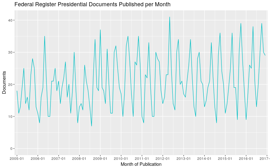
Federal Register Presidential Documents Published per Month
Wow, the number of presidential documents in the register fluctuates a lot! Instead of looking at time linearly, what if there is a pattern grouped by month
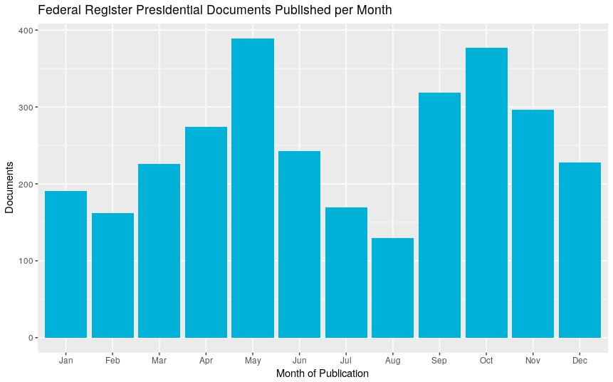
Federal Register Presidential Documents Published per Month
So the president takes it easy in the winter and summer, but kicks it into high gear in the spring and fall.
What are the top five agencies by number of documents in the federal register and how do they compare to the rest?
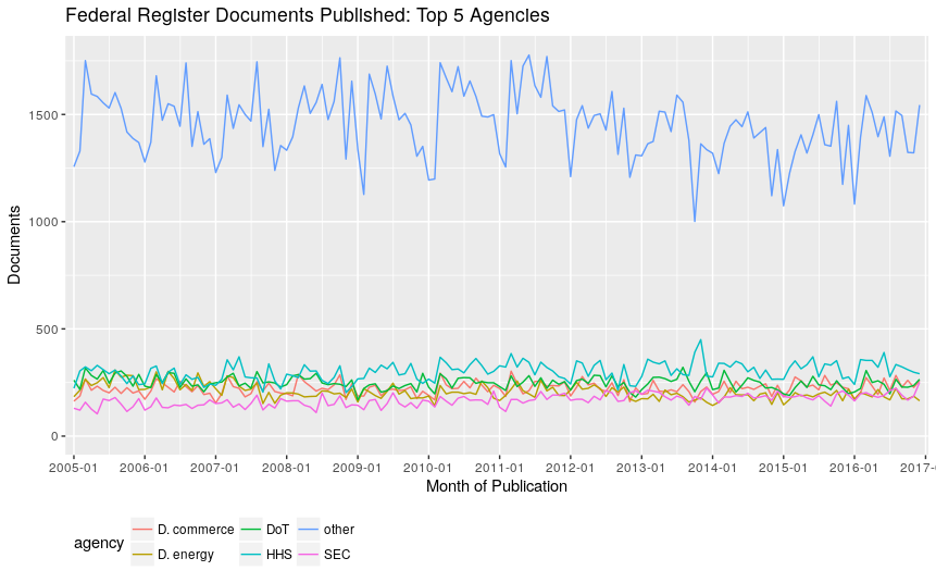
Federal Register Documents Published: Top 5 Prolific Agencies
While the top 5 agencies are somewhat close to each other, they are all dwarfed when other agencies are included. Let’s break down the document types for the top 5 agencies
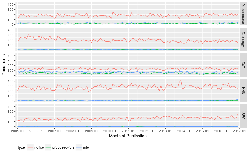
Federal Register Document Types per Agency
All agencies appear to follow the trend that the number of published notices far outweigh proposed-rules and rules. The one exception being the department of transportation, which contains the most rules and the least notices. Why this might be is beyond me!
Let’s see if we can’t depict how ephemeral people are (eg. people are promoted, administration changes, etc). So for each month, grab the top names and we’ll graph their growth.
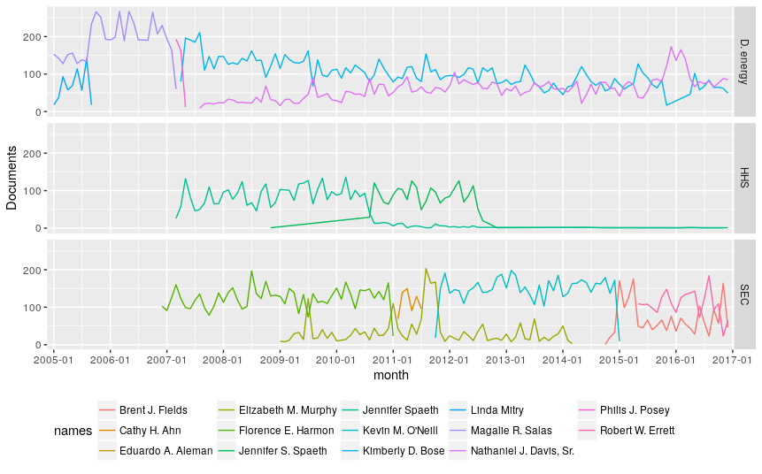
Federal Register Documents Signed by the Most Prolific Signers
Maybe I’ll figure out how to discern individuals better, but we can see those who once were prominent are replaced by someone new.
Remaining Questions
To run the XQuery transformation on 3,000 files the JVM is started and stopped 3,000 times. This is time consuming and wish there was a better way. I have stumbled across drip and ahead of time compilation of JDK9, but I haven’t had too much success with them.
Comments
If you'd like to leave a comment, please email [email protected]