
Federal Register Data Exploration with R
Published on:Table of Contents
Federal Register Data
Every year the Federal Register publishes an XML dataset, which contains daily breakdown of rules and notices that were published. In this post, I will be using the 2015 dataset, where each xml document represents a day.
Here’s a synopsis of what’s in the federal register (from their site):
Notices
This category contains non-rulemaking documents that are applicable to the general public and named parties. These documents include notices of public meetings, hearings, investigations, grants and funding, environmental impact statements, information collections, statements of organization and functions, delegations, and other announcements of public interest.
Proposed Rules
This category contains proposed regulations. These documents announce and explain agencies’ plans to solve problems and accomplish goals, and give interested persons an opportunity to submit comments to improve the final regulation. It also includes advance notices of proposed rulemaking, petitions for rulemaking, negotiated rulemakings, and various proposed determinations and interpretations.
Final Rules
This category contains regulations that apply to the general public and have final legal effect. It also includes interim final rules, direct final rules, and various determinations, interpretive rules, and policy statements. The documents cite to the Code of Federal Regulations, which contains the codified text of final rules, and is published annually in 50 titles.
Presidential Documents
This category contains documents signed by the President of the United States. Documents include Executive Orders, Proclamations, Administrative Orders, Presidential Memoranda, and other issuances of the President that are required or directed to be published in the Federal Register.
The first order of business is to solve the xml problem. Most analytical tools don’t work with xml, so we’ll need to convert it into more workable form. Since the data is somewhat non-trivial (unzipped to ~700MB) we’ll want to query from a database like Postgres because databases are analytical tools bread and butter. How this is done is a subject for another blog post but the high level flow is depicted below.
+---------+              +----------+             +-----------+
|         |  XQuery 3.1  |  better  |   custom    |           |
|   xml   +------------->+   xml    +------------>+ Postgres  |
|         |              |          | xml-to-csv  |           |
+---------+              +----------+             +-----------+
Here’s the flow in words:
- First we start with non-trivially nested xml document
- Reduce it into a desired form with XQuery 3.1
- Then using a custom written java program, convert certain xml to csv (it’s really simple, really) into a series of csv files.
- Load csv files into Postgres using pgloader
After the conversion, the data will have the following structure in the database:
- Each document represents a day
- Within a day are several issuances. Each issuance has:
- An associated department
- A number of paragraphs with a word count
- A number of people that signed the issuance
- A number of tables
- A number of presidential issuances
- Within a day are several issuances. Each issuance has:
Getting Started
I’ll be using R to analyze the data and create visuals. With each visual I’ll provide the snippet of code that generated the visual. Before we get to any visuals, though, we must connect to the Postgres data.
library(RPostgreSQL)
library(dplyr)
library(ggplot2)

# Connection info to connect to database
flexml_pg <- src_postgres(dbname = "flexml",
                          user = "integrationUser",
                          password = "integrationPassword")

# Reference the table that contains the date for each document
root <- tbl(flexml_pg, "root")

# Reference the table that contains the issuances, the agency, and what type of
# issuance
sections <- tbl(flexml_pg, "section")

# Reference the table that contains people who signed issuances
names <- tbl(flexml_pg, "name")

# Reference the table that contains paragraphs for each issuance and the number
# of words per paragraph
paragraphs <- tbl(flexml_pg, "p")

# Reference the table that contains the number of rows and cols for each
# issuance.
tables <- tbl(flexml_pg, "tbl")

# For the graphs we'll generate, the default font size is may be too hard for
# some to read, so we set the default theme to an increased size
theme_set(theme_gray(base_size = 18))
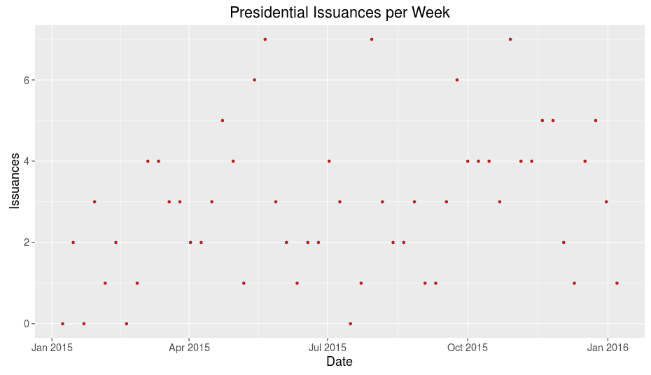
Presidential Issuances
The graph below charts the number of presidential documents there were on a weekly basis.
Presidential Issuances
# Execute raw sql because dplyr freaks out about the "FROM" keyword in extract
presql <- "SELECT EXTRACT(WEEK FROM date) AS WEEK, SUM(presidential) FROM ROOT GROUP BY week"
tbl(flexml_pg, sql(presql)) %>% collect %>%
  ggplot(aes(as.Date(week * 7, origin="2015-01-01"), sum)) +
  geom_point(color="firebrick") +
  labs(title="Presidential Issuances per Week", y="Issuances", x="Date")
Except at the extreme ends (representing the New Years), the graph depicts pretty uncorrelated data, so the number of presidential documents per week is essentially random.
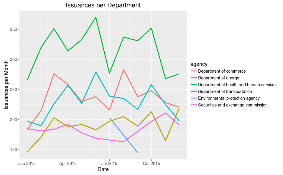
Issuances per Agency
What agencies are the most prolific issuers? The below graph takes the top 5 agencies per month and graphs the number of issuances.
Agency Issuances
secsql <- sprintf(
  "WITH p AS (
    SELECT EXTRACT(MONTH FROM date) AS month, agency, COUNT(*) as count FROM root
    INNER JOIN section ON section.xmlid = root.xmlid
    GROUP BY month, agency
), p2 AS (
    SELECT month, agency, count,
        rank() OVER (PARTITION BY month ORDER BY count DESC) as rank
    FROM p
)
SELECT * FROM p2 where rank < 6")

tbl(flexml_pg, sql(secsql)) %>% collect %>%
  ggplot(aes(as.Date(paste("2015", as.character(month), "01", sep="-")), count, group=agency, color=agency)) +
  geom_line(size=1.5) +
  labs(title="Issuances per Department", y="Issuances per Month", x="Date")
This graph is not impressive until you take the count of how many agencies have published in the Federal Register:
sections %>% select(agency) %>% distinct() %>% collect() %>% nrow()
There are 183 agencies and only six agencies are ever considered in the “Top 5” on a month to month basis across the year. An interpretation is that the other agencies are not close to the fore-runners or at least don’t fluctuate enough to gain a spotlight.
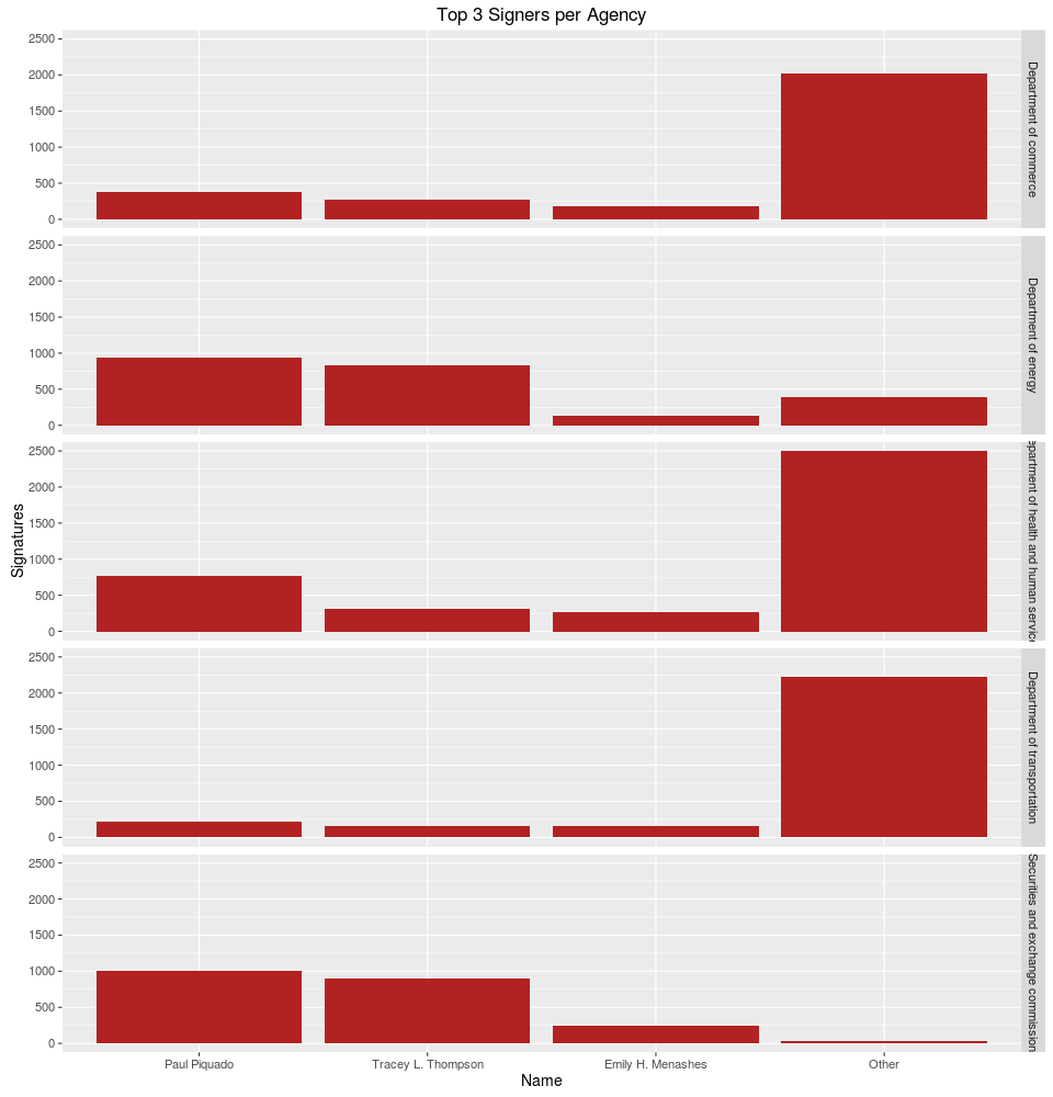
Top Signers for Agencies
Who signs off on these issuances?
Agency Signers
# Unlike the last query, we're just going to take the top five agencies for the
# year based on number of issuances.
topAgencies <- inner_join(sections, names) %>%
  group_by(agency) %>%
  tally() %>% top_n(5) %>%
  collect %>% .[["agency"]]

# Per agency calculate the top three signers and lump the other signers into an
# "Other" category
agents <-
  inner_join(sections, names) %>%
  filter(agency %in% topAgencies) %>%
  group_by(agency, name) %>%
  tally(sort = TRUE) %>%
  collect() %>%
  group_by(agency, name = factor(c(name[1:3], rep("Other", n() - 3)),
                                 levels=c(name[1:3], "Other"))) %>%
  tally(n)

# The agency names are long so we decrease font size
theme_set(theme_gray(base_size = 14))

agents %>% ggplot(aes(name, n)) +
  geom_bar(stat="identity", fill="firebrick") +
  facet_grid(agency ~ .) +
  labs(title="Top 3 Signers per Agency", x="name, y="Signatures") +
Wow, to me this is unexpected. For the top five agencies, the same three people are the top signers, and in the same order. A bit of Googling revealed their positions to be secretaries or directors, which makes sense. Still very surprising to find that the three top signers are basically the only signers for the Department of Energy and the Securities and Exchange Commission. Poor Paul, looks like signs his name several thousand times a year!
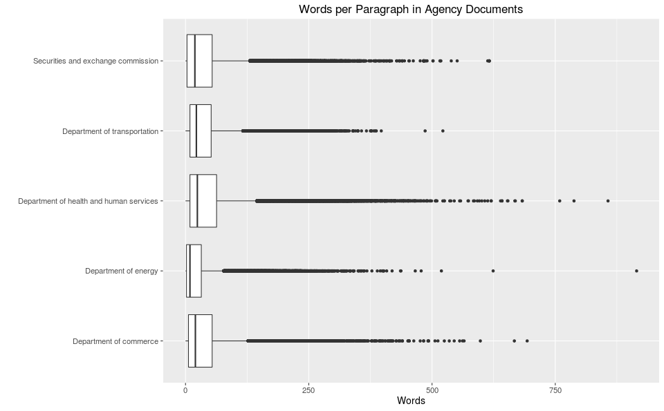
Words per Paragraph per Agency
Are documents issued by one agency more verbose than another?
Word Count by Agency
words <-
  inner_join(sections, paragraphs) %>%
  filter(agency %in% topAgencies) %>%
  group_by(agency) %>%
  select(agency, words)

words %>% collect %>%
  ggplot(aes(agency, words)) +
  geom_boxplot() +
  coord_flip() +
  labs(title="Words per Paragraph in Agency Documents", x="", y="Words")
Nope, looks pretty even, though one could say that typically, the Department of Energy, uses fewer words per paragraph, yet the same agency also contains a monster paragraph of a thousand words!
Tables Statistics
How many rows and columns do tables typically have?
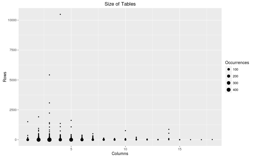
Complexity of Tables
tables %>%
  collect %>%
  ggplot(aes(columns, rows)) +
  geom_count() +
  scale_size_area() +
  labs(title="Size of Tables", x="Columns", y="Rows") +
  scale_size("Occurrences")
On average most tables are simple (few number of columns and rows). Very rarely do we see complex tables (>10 columns) and rarely do we see large tables (>1000 rows).
Comments
If you'd like to leave a comment, please email [email protected]
Wow interesting use of Federal Register data!