
Visualizing Ann Arbor Incidents
Published on:Table of Contents
Not to waste any time at all, I’ve compiled a list of incidents reported by the University of Michigan’s police and plotted their latitude and longitude on a map.
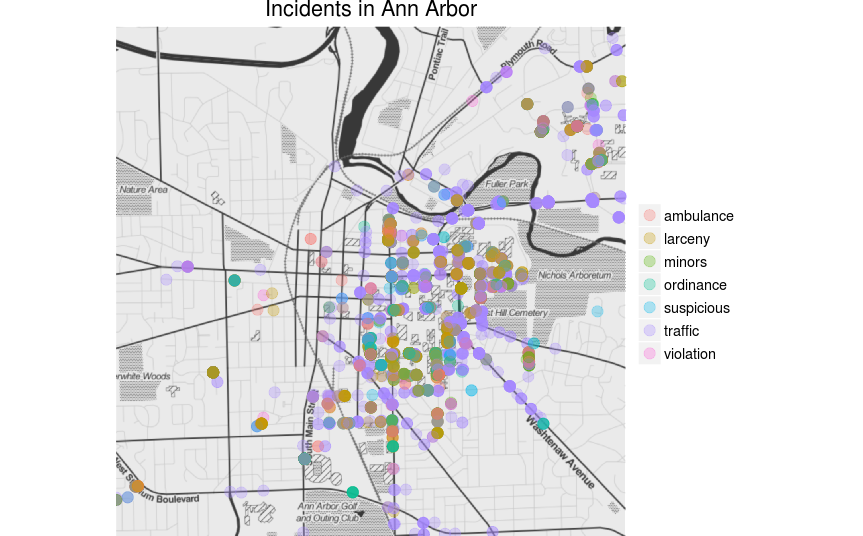
Ann Arbor Reports Mapped by Location
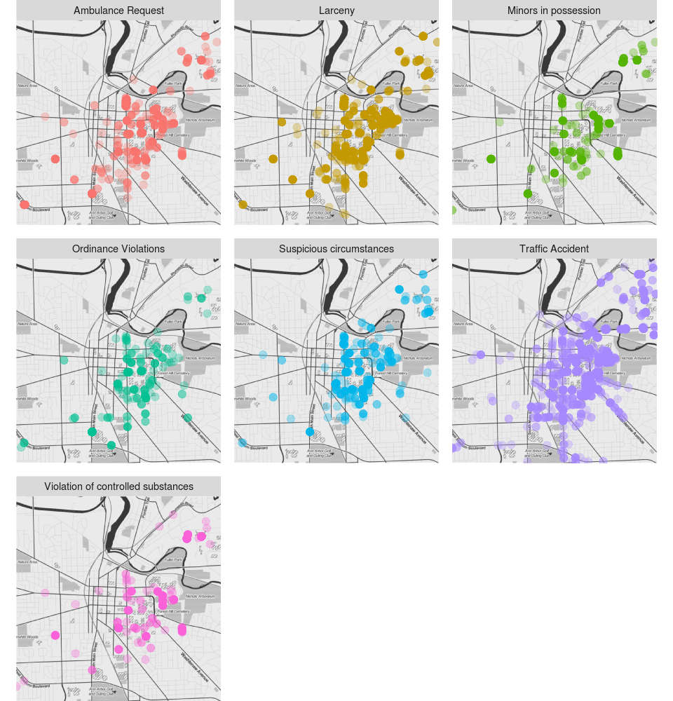
Ann Arbor Reports Mapped by Location and Type
Draw what conclusion you may. I found them unsurprisinging. Most incidents happen in around campus.
The Process
To gather all the data, I first used a script to get a thousand day’s worth of incidents from University of Michigan police department’s daily incident log. The result was a single JSON file containing all the incidents.
Couple problems with the data. The biggest is that the data didn’t contain longitude and latitude of the incidents, only the addresses. This means that if I wanted to map all 14 thousand incidents, I’d have to geocode them. Geocoding 14,000 addresses is no small feat. Google Maps only allows for 2,500 requests a day. With 14,000 addresses that would take nearly a week to accomplish.
Luckily, there’s a DIY approach: using Postgres’s PostGIS extension with the TIGER data set. Turns out, this was a nightmare to install. After searching for hours, I found a script that I had to download and heavily modify. I had to run through the install several times because of it being misconfigured each time. Not user friendly at all, yet very impressive technology.
Unleashing the dataset on my home brewed geocoder was an error prone process, as I learned various things:
- There are bugs in the geocoder that may crash the database connection with certain addresses
- Some addresses were unable to be sanely geocoded (eg, the address would resolve in another state)
- The addresses listed in the incident may be street intersections and not street addresses
- Addresses may be ambiguous (1201 Main could refer to 1201 S Main or 1201 N Main)
So I tried cleaning up the data as best I could as I went along. Still when all is told and done it probably took me more than a week to geocode the whole dataset because of all the errors I encountered and geocoding each address took about 5 seconds, which translates into nearly a day’s worth of constant geocoding sql queries (Postgres was pegged at 100% all day).
I don’t envy services that geocode for a living. Seems tough!
The Code
Below is the python code to transform the original 14,000 incident dataset into one that contains latitude, longitude, and the normalized address for each incident.
import json
import psycopg2
from datetime import datetime

# SQL query that when given street address, will return longitude, latitude,
# normalized address, and a rating from 1 (the best) - 100 (the worst) on how
# confident gecoding completed.
query = """
SELECT g.rating,
       ST_X(g.geomout) as lon,
       ST_Y(g.geomout) as lat,
       pprint_addy(g.addy)
FROM geocode(%s || ', Ann Arbor, MI') as g
"""

# Similar to the previous geocode this one works not on street addresses, but
# on two streets and will calculate the coordinates of their intersection
intersection_query = """
SELECT g.rating,
       ST_X(g.geomout) as lon,
       ST_Y(g.geomout) as lat,
       pprint_addy(addy)
FROM geocode_intersection(%s, %s, 'MI', 'ANN ARBOR 48104') as g;
"""

# Massage the address into a more geocoding friendly address
def make_nice_address(incident):
    addr = incident.get('address')

    # If we encounter 1201 MAIN, it most definitely not 1201 N MAIN as the
    # geocoder likes to think so we mainly convert it to 1201 S MAIN, which is
    # the stadium
    if addr.upper() == '1201 MAIN':
        incident['address'] = '1201 S MAIN'
    else:
        # The geocode has troubles dealing with all the abbreviations of BLOCK
        incident['address'] = addr.replace(' BLK ', '')\
            .replace(' BLOCK ', '').replace(' blk ', '')\
            .replace(' bl ', '')
    return incident

# If there is a slash in the address then we know it is two streets so compute
# the coordinates of the intersection else the coordinates of street address
def execute_correct_query(addr, cur):
    if ' / ' in addr:
        first, second = addr.split(' / ')
        cur.execute(intersection_query, (first, second))
    else:
        cur.execute(query, (addr,))

def geocode(incident):
    addr = incident.get('address')
    try:
        # Need to put connection here to avoid "current transaction is
        # aborted, commands ignored until end of transaction block" on
        # geocode_intersection('S FOREST', 'WASHTENAW ', 'MI', 'ANN ARBOR
        # 48104'), as PostGIS break :(
        conn = psycopg2.connect("dbname=postgres user=postgres")
        with conn.cursor() as cur:
            execute_correct_query(addr, cur)
            results = cur.fetchone()
            rating, lon, lat, new_address = results
            print(datetime.now(), addr, results)
    except Exception as e:
        print(datetime.now(), "Error on " + addr + ": " + str(e))
        rating, lon, lat, new_address = 100, 0, 0, ""

    # Update the JSON element with new-found information
    incident.update({
        'rating': rating,
        'lon': lon,
        'lat': lat,
        'new_address': new_address
    })
    return incident

data = json.loads(open('data.json', 'r').read())
data = filter(lambda x: len(x.get('address', "")), data)
data = map(make_nice_address, data)
data = map(geocode, data)
data = filter(lambda x: x.get('rating') <= 80, data)

with open('/tmp/data3.json', 'w') as f:
    json.dump(list(data), f)
Finally the R code to make the graphs.
library(jsonlite)
library(dplyr)
library(ggmap)
library(ggplot2)

incidents <- fromJSON("/home/nick/temp/data3.json") %>%
  rowwise() %>%
  mutate(short = first(first(strsplit(tolower(description), "[, -/]+")))) %>%
  ungroup()

# Find the top category of incidents
topShorts <- incidents %>%
  group_by(short) %>%
  tally() %>%
  top_n(7) %>%
  collect %>% .[["short"]]

# Filter incidents to those in the top categories
incidents <- incidents %>% filter(short %in% topShorts)

# Create the base map and scatterplot
map.aa <- qmap("Ann Arbor", zoom=14, source="stamen", maptype="toner", darken=c(.3,"#BBBBBB"))
g_points <- geom_point(data=incidents, aes(x=lon, y=lat, color=short), alpha=.3, size=5)

# Show the map with all the categories
map.aa + g_points + theme(legend.title=element_blank())

# Now let's make a faceted graph. Create a mapping from category to human text
# so that the facet looks nicer. In the name of GRAPHS!
incident_type <- c(
  ambulance = "Ambulance Request",
  larceny = "Larceny",
  minors = "Minors in Possession",
  traffic = "Traffic Accident",
  ordinance = "Ordinance Violations",
  suspicious = "Suspicious Circumstances",
  violation = "Violation of Controlled Substances"
)

map.aa + g_points +
  facet_wrap(~short, ncol=3, labeller = labeller(short = incident_type)) +
  theme(panel.margin = unit(1, "lines"), legend.position="none")
Comments
If you'd like to leave a comment, please email [email protected]