
Exploring TimescaleDB as a replacement for Graphite
Published on:Table of Contents
Update: 2018-09-26: This article has been updated to clarify what I meant when I described Timescale as bloated, and a correction to the collectd’s batch insert claim (it does support a form of batch inserting)
There’s a new time series database on the block, TimescaleDB, which is an extension to Postgres. I decided to test it to see how well it fits in my monitoring stack that culminates with visualizations in Grafana. Currently, I’m exclusively using Graphite as my time series database, and I’ve been curious how Timescale stacks up against it, as Influx and Prometheus failed to match.
Not to spoil the conclusion, but I found that while much touted plain ole SQL is Timescale’s greatest strength, SQL is also its greatest weakness, so Timescale definitely can have a spot in one’s stack, but it can’t wholesale replace graphite.
Mental Model
Acquainting tech support with Graphite’s architecture has been a major pain point because Graphite is colloquially used when referring to the individual components that make up a Graphite install: Carbon, a data ingestion engine that caches metrics before writing them to per-metric Whisper files, and graphite-web, which provides an rudimentary web interface and API to the data. Below is the architecture diagram for Graphite, lifted from their Github page. You will see that even in my brief description that I was skipping components, like an optional memcached layer:
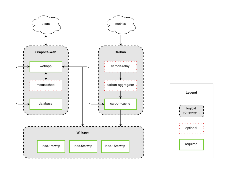
Graphite Architecture
Note: The diagram is incomplete with the new addition of a TagDB, which I’ll touch on later
When something goes wrong at a Graphite install it’s not intuitive what to check first:
- Is it one of the thousands of whisper files? Check each file with python scripts. Merging renamed metrics and deleting old metrics can be tedious.
- Is it carbon cache? If new metrics (ie: metric name) are being sent to carbon, by default, only 50 new ones are allowed per minute, so carefully crafted Grafana dashboards will look broken until enough time has passed, as new metrics will be dropped in the meantime. This and carbon-cache’s disk intensity (ssd’s are nigh a must) can be tuned, but it can be unintuitive what values are appropriate for the number of updates per second in this dance of disk vs ram utilization when compared to the postgres’s shared buffers.
- Is it graphite web? Was installed correctly? Is it talking to the correct carbon-cache? Did a plugin go bottom up and require a restart of the service?
Tech support has better use of their time than to memorize the components and how to troubleshoot each one.
Compare this with TimescaleDB. It’s postgres. People know how to manage postgres or are able to tap into the vast amount of resources on the internet for administration help.
Data Data Data
Before painting a too poor of a picture of graphite, I find how it manages data levelheaded. While one may have thousands of whisper data files, they are all fixed size, so once allocated, one knows what disk requirements are necessary. This is possible due to one setting a max retention period (like one year), with older data automatically erased. In addition, one can set multiple retention period to downsample a single metric to save space. For instance, I use 10s:6h,1m:6d,10m:1800d, which reads “save data in 10 second intervals until 6 hours, then the data is bucketed into minute intervals by averaging (configurable) the (6) 10 second intervals that make up a minute, and after 6 days group minutely data into 10 minute buckets and keep those around for 5 years.” All told, for this retention policy, each whisper file consumes 3.1MB, which I find to be fairly incredible as there is over 250k 10 minute intervals in 5 years (one whisper data point is only 12 bytes).
My small home graphite install is 7GB with 2310 metrics representing 600 million data points over 5 years. To me, this is an incredible feat.
The biggest downside of carbon data retention is changing your mind (eg: one needs finer resolution) won’t change any metrics already created. One will need to whisper-resize appropriate files which can be easy to forget or mess up.
Back to doling out laurels. Inserting data into carbon could not be any easier, below we’re telling carbon that we see 10 unique clients at the current date:
echo "pihole.unique_clients 10 $(date +%s)" >> /dev/tcp/localhost/2003
Everyone that’s seen this groks it fairly quickly and can adopt it for their own scripts. There is no barrier to entry. And any prior entry for metric has its value overwritten, which make updates just as straightforward.
Contrast this with Timescale. Data is stored in SQL tables, which allows you to structure your data however you want, whether that be one table or many, wide or narrow, denormalized or normalized, indices galore and triggers aboard. Postgres – it’s flexible. But there are some caveats:
- Deleting data from Timescale requires intervention, so one will need the cron or systemd script provided if they need to automate it. One may have limited disk space.
- Timescale does not downsample data
- Most Timescale installs will be much more bloated after 5 years unless one employs surrogate keys to reduce duplication from repeatedly storing “pihole.unique_clients” in a column, but this normalization has its own downsides (increased insert and query complexity). [1]
- Have to insert data via
psqlcli (or postgres library in an application) which will require authentication hoops to jump through. - Timescale will allow duplicates rows and create ambiguous situations (was the hard drive 40°C or 50°C?)
But each of these points can have a positive spin on them:
- Business requirements will change so one can fine tune deleting data on a need to do basis or some other logic.
- It may not be clear what aggregation is most appropriate when downsampling (graphite defaults to average), so by not downsampling, one keeps the raw data to determine what aggregation is most appropriate at time of query.
- The beauty of SQL is that you can decide what’s right for you. Hopefully a denormalized form is appropriate, but anything is possible when JOINs are at your fingertips.
- No unauthenticated access to the database. One should create service accounts with locked down access. Also with SQL inserts, one can use parameters to nullify injection, while graphite needs special characters removed in each metric name segment prior to transmission to prevent unpredictable errors during analysis.
- If your business requirements disallow duplicates, you can dictate this through unique indices on necessary columns and upsert all your data (though at the cost of disk space for additional index and insert complexity as one needs to include the “ON CONFLICT DO” clause).
Setting Up
At home, I have the luxury of farming the onus of installation to Docker. Both Timescale and Graphite have official docker images. This simplifies getting started, but if we compare docker image sizes (Timescale: 15-30MB vs Graphite: 341MB), it helps shed light on how heavyweight each application is.
But let’s set aside docker for a moment and focus on installing in an enterprisey environment like enterprise linux.
Timescale is easy it’s about 2 lines of yum and 1 postgres configuration line change.
Graphite not so much:
- Download python 2.7 source
- Ensure all appropriate devel libraries are downloaded like openssl-devel
- Compile and install this python 2.7 into a directory
- Even if you’re not using the web ui you still need to install cairo-devel
- Pip install all the requirements
- Execute a django incantation (I think it sets up some kind of database)
- Configure a reverse proxy like gunicorn or nginx (fastcgi)
- Add init scripts / systemd.
It’s easy to slip up and omit a dependency, and you won’t know it by the opaque errors that are logged.
Concerning upgrades, for graphite, one will need to closely track the release notes to see what dependencies need to updating (like Twisted or Django), so things can get tricky, though with Docker, upgrades are seamless as the internal whisper format has never changed. Whereas for Timescaledb, one can use any standard postgres upgrade mechanism: pg_dump and restore, pg_upgrade, or logical replication.
On Tags
Within the last year, Graphite has gained support for tagging metrics. Tags allow one circumvent querying purely on the hierarchy of a metric name. Tags are a nice addition, as it’s now easier to cobble together disparate systems based on a tag. For instance you could have multiple projects that report on temperature, and now it doesn’t matter where in the hierarchy those temperatures are stored, one can select them with a simple graphite query:
seriesByTag('sensor_type=Temperature')
I bring up tags for one good reason. Tags need a TagDB (a component missing from architecture diagram). The default TagDB is sqlite. However, according to an official Graphite maintainer, any serious interest in tags should use an external db like postgres, mysql, or redis. Now we have two systems: graphite-web + carbon + whisper + all those dependencies + postgres vs just postgres.
Using tags is entirely optional, but come at a cost of an additional component to manage. Not to mention, if one were to tack on another tag to a metric, it will create an entirely new metric and I haven’t figured how one migrates the old data. I just end up resigning data to rot. For Timescale, one relies on the standard ALTER TABLE syntax when adding / removing columns.
Querying
Graphite reigns supreme when it comes to querying. It’s whole purpose is to provide an HTTP API over time series data, so it comes packed with functions. I’ve been writing Graphite functions for probably over three years and I’m routinely surprised at how powerful they are (like two months ago when I finally used reduceSeries).
I wrote an application that will export hardware sensor data from my Windows machines called OhmGraphite. We’re going to use it to drive our example, as it’s the only metrics agent I know that has a nice integration with Timescale. Below is a graph we’ll create of the temperature for the hottest two hard drive on average:
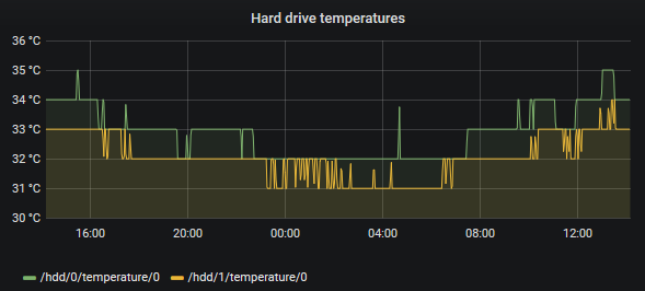
Grafana panel showing hard drive temperatures
Here is the Graphite query:
seriesByTag('sensor_type=Temperature', 'hardware_type=HDD')
  | highest(2, 'average')
  | aliasByTags('name')
It’s 3 concise and readable lines. I can easily switch from highest(2, 'average') to highest(5, 'stddev') to see the top 5 hard drives with the highest standard deviation. Extremely powerful, extremely simple.
The same can’t be said for Timescale:
-- Get the temperature data for each hard drive grouped into time buckets
WITH data AS (
    SELECT
        identifier,
        time_bucket ('$__interval', time) AS "btime",
        AVG(value) as avg_data
    FROM ohm_stats
    WHERE $__timeFilter(time)
        AND sensor_type = 'Temperature'
        AND hardware_type = 'HDD'
    GROUP BY btime, identifier
),

-- Compute the overall average temperature from the data buckets and
-- give that hard drive a rank
ranks AS (
    SELECT
        identifier,
        RANK() OVER(ORDER BY avg(avg_data) DESC) as rnk
    FROM data
    GROUP BY identifier
),

-- Since the hard drive may not have data for the entire interval,
-- we need to create a gap filling function
 period AS (
    SELECT time_bucket ('$__interval',  no_gaps) AS "btime"
    FROM generate_series($__timeFrom()::timestamptz, $__timeTo(), '$__interval') no_gaps
)

-- Then for each top hard drive, create a series with just the time
-- and the identifier (cross join) and then selectively grab the
-- data that's available (left join)
SELECT
    $__time(period.btime),
    data.avg_data,
    ranks.identifier AS "metric"
FROM
    period
    CROSS JOIN ranks
    LEFT JOIN data ON
        period.btime = data.btime
        AND data.identifier = ranks.identifier
WHERE ranks.rnk <= 2
ORDER BY period.btime
Wow. It took me an embarrassing amount of time to craft this query. We’re talking hours of tweaking. I’m cautiously optimistic that there are ways to improve this query because a 10-15x increase in a query statement length is not something I look forward to maintaining. Changing the aggregation from average to something like standard deviation, or returning the top 5 instead of 2 isn’t apparent. Grafana variables make it a little easier to inject these types of changes. Since I said “inject” in the context of SQL, I must now mention that postgres user grafana utilizes to interact with Timescale should be greatly restricted, else expect someone to delete all the data!
Aside: while I have not done a deep performance analysis, both queries are within spitting distance of each other in the time it takes to return results. I’m secretly hoping that if I am able to migrate entirely to Timescale that I’d have more predictable memory usage, and less resource usage in general, but I can’t even speculate on that at the moment.
All this SQL written does give a bit of flexibility. Postgres aggregate and window functions are at our fingertips. For instance, we can graph how the rank of the hottest hard drives change throughout time (eg: the 5th hottest hard drive on average may have intervals where it is the hottest or coldest), by simply tweaking the final SELECT statement from the previous section to rank each hard drive at each interval:
-- Then for each top hard drive, create a series with just the time
-- and the identifier (cross join) and then selectively grab the
-- data that's available (left join)
SELECT
    period.btime AS "time",
    RANK() OVER (PARTITION BY period.btime ORDER BY data.avg_data DESC) brnk
    ranks.identifier AS "metric",
FROM
    period
    CROSS JOIN ranks
    LEFT JOIN data ON
        period.btime = data.btime
        AND data.identifier = ranks.identifier
ORDER BY period.btime
This is where we start thinking about creating a function to extract all this functionality so we can stop repeating ourselves, but I’m going to stop on the querying part. If you’re interested in what’s next, here’s an example of a postgres function. I just wanted to convey that crafting queries in grafana is 10x easier with graphite than timescale. You’ll need to write your own scaffolding to make it easier with timescale. At least, the query language is only SQL, which more business analysts are privy to, unlike some other custom time series database languages!
Hopefully soon the Timescale team will add in much needed features like gap filling by previous value, as current SQL workarounds are obtuse. Ideally, I’d like to see a translation document of Graphite functions to postgres SQL, as Graphite is the query gold standard.
While I can’t laud Graphite enough in the context of Grafana, Timescale does have a trick up its sleeve. By virtue of being just Postgres, it integrates more readily into traditional BI programs like Tableau that can query the database directly. I was able to get graphite data into a state Tableau could query by using an intermediate SQL database (go figure) and writing an application that formats graphite csv output into appropriate sql statements. This method is not something I recommend.
Conclusion
- I have tiny scripts (like Robust systemd Script to Store Pi-hole Metrics in Graphite that I’m unlikely to migrate off graphite, due to the script not being important and I’d need to format the queries as SQL statements (I’d need to figure out how I’d want to access psql: docker or install via package manager)).
- Timescale is new enough not to have wide adoption amongst collection agents. I can’t migrate my post Monitoring Windows system metrics with Grafana to Timescale, as telegraf doesn’t support reporting to Timescale (maybe it is time I look past telegraf).
- Collectd does support writing to postgres,
though reviewing the code – it doesn’t batchCollectd does support batch inserts through theINSERTstatements most likely leading to less than stellar performance. I may have to end up writing a collectd plugin as a proof of concept.CommitIntervalconfig. - The only thing I have actually writing to Timescale is OhmGraphite
- Thus getting high quality support among collection agents is Timescale’s first hurdle
- The next step for Timescale is making queries more succinct and readable without forcing the user to create the scaffolding.
- Graphite can’t compare in ease of setup, administration, security, and sheer man hours spent in creating postgres.
- Graphite has greatly optimized ease of insertion and small disk footprint (though disk write footprint is bit of a different story)
So it’s bit of a wash. Depending on the situation, graphite or Timescale is appropriate. Not everything can insert into Timescale, but not everything can query graphite.
This article can be discussed on Hacker News too
Update 2018-09-26
Calling a TimescaleDB installation bloated may be amplifying the differences too much when comparing against Graphite, but I don’t find it a gross exaggeration. If we think of a metric series, there are essentially three components: an x and y pair, and a name. One of the redeeming features of Graphite is the condensed data format where each x and y pair is only 12 bytes. The metric name doesn’t require any storage because it is the file name. This is how graphite can cover 600 million data points covering 5 years in 3.1MB with appropriate downsampling as demonstrated in the post.
Replicating this schema with postgres, one could do:
CREATE TABLE pihole_unique_clients (
  time  TIMESTAMPTZ NOT NULL,
  value REAL NULL
);

SELECT create_hypertable('pihole_unique_clients', 'time');
Some notes:
- This sets up each pair to be the same size as Graphite (12 bytes)
- Graphite stores the time as unix time in seconds (4 bytes)
- There is not a postgres timestamp format that consumes 4 bytes, so I had to switched to
REALinstead ofDOUBLEfor the purpose of this example to achieve 12 byte rows - While TimescaleDB does allow for a 4 byte integer as the ’time’ (so one can switch back to
DOUBLEto be equivalent to graphite), in my opinion, you give up too much in terms of intuitiveness in querying and inserting. - The 12 byte rows isn’t entirely accurate for postgres due to index size and internal row bookkeeping
- This also requires that each metric be it’s own table, which is extremely unrealistic, but for the sake of example let’s continue
Using this table, let’s insert 100k seconds into the db and calculate the size
INSERT INTO pihole_unique_clients
  SELECT *, 1 AS value
  FROM generate_series(now() - interval '100000', now(), '1 second');

SELECT hypertable_relation_size('pihole_unique_clients');
The result is 8.2MB. Thus storing 2.5x fewer metrics requires more than twice the space, which translates into ~5x efficiency decrease between TimescaleDB and Graphite (hence my usage of the word “bloat”). What’s more is that this is nearly a best case scenario for Timescale. When the metrics are not known beforehand, most will opt into a narrow table format where the name (or some other variable like “location”) of the metric is duplicated on every row (and may be indexed as well), like so:
CREATE TABLE pihole (
  time  TIMESTAMPTZ NOT NULL,
  name TEXT NOT NULL,
  value REAL NULL
);
Narrow tables like this will only expound the difference between Timescale and Graphite due to the repetition. It would be an interesting to determine how wide a table must be of only DOUBLE columns (+ time column) to match the same efficiency, as graphite using the same timestamp across metrics can be seen as a form of repetition. As for the experiment, I’d suspect the breakeven point in disk space efficiency around 15-20.
But please don’t get caught up in my fascination with disk space usage. TimescaleDB will never be able to compete with a data format that has been optimized for time series and that should not be seen as a bad thing. TimescaleDB has enough inertia that focus should be spent on other features.
Comments
If you'd like to leave a comment, please email [email protected]
Without ambition to prove my comments: - most of the conclusions about TimescaleDb are wrong in this article…eg. automated data retention is already there, duplicates are easy to manage or on ingestion and via UNIQUE constraint etc… - generally I advice to learn SQL…queries are really bad - flexibility of SQL is generally unbeatable
Hello! Not sure how the conclusions are wrong. I’m very positive when it comes to TimescaleDB. I like it!
Cheers
for the data you retain over 5 years, can you create comparison charts for the data comparing dates from current year to dates prior year, or current year to 3 years ago? For example if you were capturing temp sensor data and wanted to chart daily (per hour temps) for june in current year and over lay daily temps for june in prior year.
Looking at doing something similar and trying to determine which TSDB to use. I will be keeping data indefinitely at this point. I will only end up with a max of 100 sensors sending 2-3 metrics per sensor max on average ( 1 sensor may have 1 metric, another sensor may have 5 metrics).
Thank you for this post, I found your points very helpful.